Introduction to quantum computing and the surface code
references: arXiv:0904.2557, arXiv:1208.0928
(This is the content of a talk I gave to other students in our department, most of whom have no background in quantum computing; hence the introduction and lightness on details of the surface code.)
Before talking about the surface code, I’ll introduce the fundamentals of quantum computing.
Quantum computing: The evaluation of quantum circuits in polynomial time.
Background on quantum computing
State A state is a d-dimensional vector in a complex Hilbert space ℋd. We require that the states are normalised to unity.
Qubit A qubit is a “two-level system”. This means it is a state with d = 2.
We are doing quantum mechanics, so we use bras and kets for vectors, and we distinguish some particular bases,
$$ \begin{aligned} |0\rangle &= \left( \begin{array}{c} 1 \\ 0 \end{array} \right), \\ |1\rangle &= \left( \begin{array}{c} 0 \\ 1 \end{array} \right). \end{aligned} $$
Note that these two vectors form a basis for ℋ2. We call this basis the standard basis. All bases here will are assumed to be orthonormal.
Written in the standard basis an arbitrary qubit is then given by
$$ \begin{aligned} |\psi\rangle = \alpha |0\rangle + \beta |1\rangle. \end{aligned} $$
For a ket |ψ⟩ the bra is given by ⟨ψ| = (|ψ⟩)†, where † means take the conjugate tranpose. So we write the inner product as ⟨ψ|φ⟩ and the outer product as |ψ⟩⟨φ|.
We will also refer to the so-called Hadamard basis, which is
$$ \begin{aligned} |+\rangle &= \frac{1}{\sqrt{2}}\left(|0\rangle + |1\rangle\right), \\ |-\rangle &= \frac{1}{\sqrt{2}}\left(|0\rangle - |1\rangle\right). \end{aligned} $$
Qubits We can form a state containing multiple qubits using the tensor product. Verbosely, one may write:
$$ \begin{aligned} |0\rangle \otimes |0\rangle \otimes \cdots \end{aligned} $$
but we will shorten this to:
$$ \begin{aligned} |00\cdots\rangle &= |0\rangle \otimes |0\rangle \otimes \cdots. \end{aligned} $$
The dimension of the Hilbert space of this state is ℋ2n, where n is the number of terms in the tensor product: the number of qubits.
Operator An operator (sometimes called a gate), M, is a 2n × 2n-dimensional matrix with elements in ℂ. We require that the operators be unitary; i.e. that MM† = M†M = 1 (this requirement comes from the fact that any such operator should preserve the norm of the states).
A note on notation Given a multi-qubit state, |abcd⟩, we can perform a single-qubit operator M on each of these qubits by constructing the appropriate tensor product of matrices, M ⊗ M ⊗ M ⊗ M, and then acting this on the state. We will often write this more concisely as M1M2M3M4|abcd⟩, indicating which qubit the operator acts on.
Pauli Matrices These play a key role in the surface code. We will define them as
$$ \begin{aligned} X &= \left( \begin{array}{cc} 0 & 1 \\ 1 & 0 \end{array} \right), \\ Z &= \left( \begin{array}{cc} 1 & 0 \\ 0 & -1 \end{array} \right), \\ Y &= \text{i}XZ. \end{aligned} $$
Note that they all square to 1. We will only be interested in the action of X and Z, so note:
$$ \begin{aligned} X|0\rangle &= |1\rangle, \\ X|1\rangle &= |0\rangle, \\ Z|+\rangle &= |-\rangle, \\ Z|-\rangle &= |+\rangle. \end{aligned} $$
And furthermore, we have XZ = −ZX (these operators anticommute).
Measurement Quantum mechanics prescribes that for an arbitrary qubit (written in the standard basis),
$$ \begin{aligned} |\psi\rangle &= \alpha|0\rangle + \beta|1\rangle, \end{aligned} $$
then measuring this qubit gives the state |0⟩ with probability |α|2 and state |1⟩ with probability |β|2.
More generally we can make projective measurements, wherein we project a state |ψ⟩ into a particular basis. It is common to observe that, in terms of eigenvalues and eigenvectors (by the spectral decomposition theorem),
$$ \begin{aligned} X &= |+\rangle\langle +| - |-\rangle\langle -|, \\ Z &= |0\rangle\langle 0| - |1\rangle\langle 1|, \end{aligned} $$
and therefore make statements such as “measure in the X basis”, where this means to project the qubit into the basis {|+⟩, |−⟩}.
Quantum circuits
An example quantum circuit:
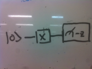
This enacts the operator X on the state |0⟩, and we “measure” this state at the end of the circuit in the Z basis.
The outcome of this circuit is the state |1⟩ with certainity.
Let $H = \frac{1}{\sqrt{2}} \left( \begin{array}{cc} 1 & 1 \\ 1 & -1 \end{array} \right)$ and $C_X = \left( \begin{array}{cccc} 1 & 0 & 0 & 0 \\ 0 & 1 & 0 & 0 \\ 0 & 0 & 0 & 1 \\ 0 & 0 & 1 & 0 \end{array} \right) = \left( \begin{array}{ccc} 1 & & \\ & 1 & \\ & & X \end{array} \right)$.
A more complicated circuit:
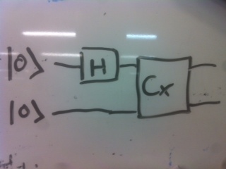
The outcome of this circuit is the state |00⟩ + |11⟩. This is infact an entangled state.
Universal quantum computation
Previously I described quantum computation as the evaluation of any circuit in polynomial time i.e. we could choose any unitary operations we like.
Infact, it turns out that, due to a standard theorem (Solovay-Kitaev theorem), that if we can perform the gates {H, S, T, CX}, then we can approximate any unitary matrix (acting on the qubits involved), and hence perform any computation. (It’s not particularly important what the S and T gates are, for our purposes.)
Error correction
A natural question is - “Do we have quantum computers?”, and the answer is, “not yet”. The reason is that quantum states are decliate; they need to be well isolated from the environment; otherwise errors occur.
Classical errors
Idea of encoding
Suppose we wanted to worry about errors in bits. We could used the repitition code,
$$ \begin{aligned} 0 &\mapsto 000, \\ 1 &\mapsto 111. \end{aligned} $$
This exact procedure - copying an arbitrary state - can’t be applied in quantum computing due to the No-Cloning Theorem: There is no matrix U such that for any arbitrary |ψ⟩
$$ \begin{aligned} U(|\psi\rangle \otimes |0\rangle) = |\psi\rangle \otimes |\psi\rangle. \end{aligned} $$
Proof. Let |ψ⟩ = α|0⟩ + β|1⟩ then apply U before and after enacting the tensor product, and note contradiction.
Quantum errors
For the moment, we will consider only errors that may occur on a single qubit, i.e. an erroneous unitary operation.
Any 2n × 2n unitary matrix can infact be expressed as a sum of (tensor products of) Pauli operators, with appropriate coefficients, so we consider the general single-qubit error operator
$$ \begin{aligned} E = \epsilon_1 I + \epsilon_2 X + \epsilon_3 Z + \epsilon_4 Y. \end{aligned} $$
(Recall that Y = iXZ.)
Of course, we can correct any of these errors by applying E†, but in so doing we would in principle need to know the coefficients. It turns out there is a better way.
The first step is to think completely differently about how we would encode a logical qubit.
Consider the operators X1, X2 and Z1, Z2, acting on two qubits. These operators commute, as XZ = −XZ (and operators acting on different qubits always commute.) The (un-normalised) eigenspace is
$$ \begin{aligned} \begin{array}{ccc} Z_1 Z_2 & X_1 X_2 & \text{Eigenvectors} \\ \hline +1 & +1 & |e_1\rangle = |00\rangle + |11\rangle \\ +1 & -1 & |e_2\rangle = |00\rangle - |11\rangle \\ -1 & +1 & |e_3\rangle = |01\rangle + |10\rangle \\ -1 & -1 & |e_4\rangle = |01\rangle - |10\rangle \end{array} \end{aligned} $$
They key is this. Consider an arbitrary two-qubit system expressed in this basis
$$ \begin{aligned} |\psi\rangle = \alpha |e_1\rangle + \beta|e_2\rangle + \gamma|e_3\rangle + \delta|e_4\rangle. \end{aligned} $$
If we impose the following constraint on this system,
$$ \begin{aligned} X_1 X_2 |\psi\rangle = \lambda_X |\psi\rangle \end{aligned} $$
then we cut out two of the possible basis states that the system could be in. For example, say λX = +1.
Then this rules out the state |00⟩ − |11⟩ and |01⟩ − |10⟩, leaving us with:
$$ \begin{aligned} |\psi\rangle = \alpha|e_1\rangle + \gamma|e_3\rangle. \end{aligned} $$
Observations:
In general we rule out half the eigenvectors when specifying a stabilizer constraint.
Suppose we enact X1X2 on this new constrained state; it will remain the same, so we can measure in this basis as often as we like, and we will continue to obtain the same eigenvalue when there are no errors.
If either qubit undergoes say a Z error, the eigenvalue λX will change. So we can detect this error. We can also correct it, by applying Z again (if we wished), as Z2 = 1.
If either qubit undergoes a X error, this is not detectable. We will still be in the +1 eigenstate of X1X2, but the coefficients will have switched.
This is a toy model.
The surface code is a system by which we can detect any single qubit error, E as before, along with several other kinds.
The surface code
We define the surface code on a k × k lattice. At each lattice site we place a qubit. For example, suppose k = 3, then we have
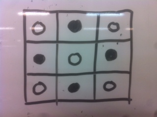
Now, we let there be two types of black cricles. Those associated with X operators, and those associated with Zs. We also label the white qubits, as these will form the quiescent state - the stable state of the surface code, and the state which we will manipulate in order to perform computation,
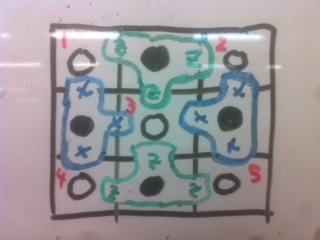
In the k = 3 system, the implementation of the surface code will enforce the following constraints (with the white qubits labelled as in the above image in red),
$$ \begin{aligned} Z_1 Z_2 Z_3 |\psi\rangle = \lambda^{(Z)}_{1,2,3}|\psi\rangle, \\ Z_3 Z_4 Z_5 |\psi\rangle = \lambda^{(Z)}_{3,4,5}|\psi\rangle, \\ X_1 X_3 X_4 |\psi\rangle = \lambda^{(X)}_{1,3,4}|\psi\rangle, \\ X_3 X_4 X_5 |\psi\rangle = \lambda^{(X)}_{3,4,5}|\psi\rangle. \end{aligned} $$
Any implementation of the surface code enforces these constraint at every time step.
In our lattice here, we have 5 data qubits, and 4 measurement qubits. We showed that there are 4 constraints coming from the 4 data qubits, and as we claimed earlier each of these halve the state space, so the resulting state space has dimension 25/24 = 2. In other words, it encodes one qubit.
Our goal now is to define logical operations on this qubit. In a much larger surface code (and with some modifications to the way logical qubits are encoded on the lattice), it is possible to define all the logical operations necessary to perform universal quantum computation, but here we’ll only look at XL and ZL.
Consider an X on data qubit 4. This operation commutes with the X stabilizers, but will be detected by the Z stabilier to the right. Consider then the operation XL = X4X5. This operation commutes with all the stabilizers, and cannot be written in terms of any of them.
So by performing these operators we have obtained |ψX⟩ = XL|ψ⟩ - we’ve manipulated one of the degrees of freedom.
Similarly, we can define ZL = Z2Z5. Note that this anticommutes with XL.
So we’ve exhibited some logical operators.
Surface code facts and final comments
Tolerant to a 1% error rate in the physical qubit operations,
Logical qubits in the code look a bit different; they are defined with respect to “defects” in a much larger lattice.
The estimate in 2012 was that ~14,500 phsyical qubits would be necessary to build one logical qubit.
In order to factor a 2000 bit number we would require 1 billion qubits.
I’ve left out a lot of details regarding how errors are corrected - this is not trivial, and it’s actually interesting.
I’ve not commented on all the types of errors that the surface code corrects against.
More information
There’s the recent surface code paper:
a fantastic recent comprehensive review:
there’s a recent video from John Martinis:
there’s even some code to go and calculate your own surface code error rates!