Quantum neural networks
(This post requires a background in the basics of quantum computing (and neural networks). Please have a read of the first part of Introduction to quantum computing and the surface code if you’d like to get up to speed on the quantum parts, Neural networks and Deep Learning is a good introduction to the other part.)
Recently, I’ve been spending a lot of time thinking about machine learning, and in particular deep learning. But before that, I was mostly concerning myself with quantum computing, and specifically the algorithmic/theory side of quantum computing.
In the last few days there’s been a flurry of papers on quantum machine learning/quantum neural networks, and related topics. Infact, there’s been a fair bit of research in the last few years (see the Appendix at the end for a few links), and I thought I’d take this opportunity to have a look at what people are up to.
The papers we’ll be discussing are:
- arXiv:1612.01045 - Quantum generalisation of feedforward neural networks by Wan, Dahlsten, Kristjánsson, Gardner and Kim.
- arXiv:1612.01789 - Quantum gradient descent and Newton’s method for constrained polynomial optimization by Rebentrost, Schuld, Petruccione and Lloyd,
- arXiv:1612.02806 - Quantum autoencoders for efficient compression of quantum data by Romero, Olson and Aspuru-Guzik,
But first, let’s take a look at the paper that got me interested in machine learning in the first place!
arXiv:1307.0411 - Quantum algorithms for supervised and unsupervised machine learning
The paper, Quantum algorithms for supervised and unsupervised machine learning by Lloyd, Mohseni and Rebentrost in 2013, was one of my first technical exposures to machine learning. It’s an interesting one because it demonstrates that for certain types of clustering algorithms there is a quantum algorithm that exhibits an exponential speed-up over the classical counterpart.
Aside: Gaining complexity-theoretic speed-ups is the central task of (quantum) complexity theory. The speedup in this paper is interested, but it “only” demonstrates a speed-up on a problem that is already known to be efficient1 for classical computers, so it doesn’t provide evidence that quantum computers are fundamentally more powerful than classical ones, by the standard notions in computer science.
The Supervised clustering problem that is tackled in the paper is as
follows:
Given some vector u⃗ ∈ ℝN, and two sets of vectors V and W, then given M representative samples from V: v⃗j ∈ V and w⃗k ∈ W, figure out which set u⃗ should go in to, by comparing the distances to these vectors.
In pictures it looks like so:
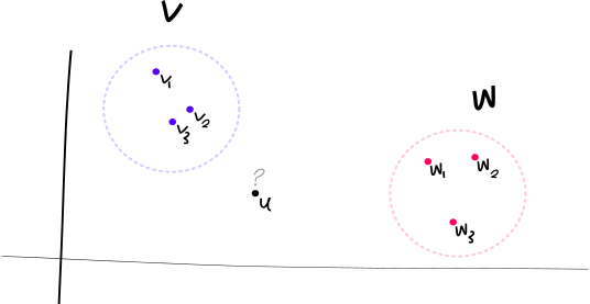
Classically, if we think about where we’d like to put u⃗, we could compare the distance to all the points $\vec{v_1}, \vec{v_2}, \vec{v_3}$ and to all the points $\vec{w_1}, \vec{w_2},\vec{w_3}$. In the specific example I’ve drawn, doing so will show that, out of the two sets, u⃗ belongs in V.
In general, we can see that, using this approach, we would need to look at all M data points, and we’d need to compare each dimension of the N dimensions of each vector $\vec{v_j}, \vec{w_k}, \vec{u}$; i.e. we’d need to look at at least M × N pieces of information. In other words, we’d compute the distance
By looking at the problem slightly more formally, we find that classically the
best known algorithm takes “something like”2 poly(M × N) steps,
where “poly” means that the true running time is a polynomial of
M × N.
Quantumly, the paper demonstrates an algorithm that lets us solve this problem in “something like” log (M × N) time steps. This is a significant improvement, in a practical sense. To get an idea, if we took 100 samples from a N = 350-dimensional space, then M × N = 35, 000 and log (M × N) ≈ 10.
The quantum algorithm works by constructing a state in a certain state so that, when measured, the distance that we wanted, d(u⃗, V), is the probability that we achieve a certain measurement outcome. In this way, we can build this certain state, and measure it, several times, and use this information to approximate the required distances. And, the paper shows that this whole process can be done in “something like” a running time of log (M × N).
There’s more contirbutions in the paper than just this; so it’s worth a look if you’re interested.
arXiv:16.12.01045 - Quantum generalisation of feedforward neural networks
So this paper is pretty cool. We can get a feel for what it’s doing by first considering the following network:
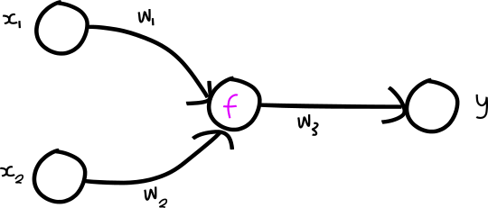
This network has two inputs, x1, x2, three learnable weights, w1, w2, w3, one output value y, and an activation function f.
Classically one would feed in a series of training examples (x1, x2, y) and update the weights according to some loss function to achieve the best result for the given data.
Quantumly, there are some immediate problems with doing this, if we switch the inputs x to be quantum states, instead of classical real variables.
The problems are:
- Quantum operations need to be reversible; f as written is not (at the very least, it takes two inputs and squashes them down to one output).
- Quantum states need to be normalised; so multiplying them by a single arbitrary weight won’t be productive.
- You can’t copy arbitrary quantum states due to the No-Cloning theorem, so this restricts the type of networks that can be written down.
The way this paper solves these problems is to transition Figure 2 from a classical non-reversible network to a reversible quantum one:
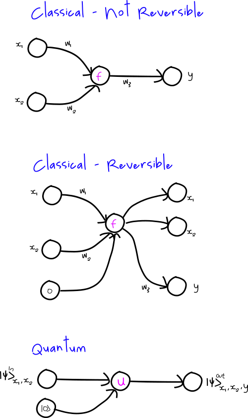
The final network takes in an arbitrary quantum state of two qubits, x1, x2, and then adjoins an ancilla state |0⟩, applies some unitary operation U, and emits a combined final state |ψ⟩x1, x2, yOut where the final qubit y contains the result we’re interested in.
At this point, one might reasonably ask: How is this different to a quantum circuit? It appears to me that the only difference is that U is actually unknown, and it is trainable! Note that this is also a somewhat radical difference from classical neural networks: there, we don’t normally think of the activation functions (defined as f above) as trainable parameters; but quantumly, in this paper, that’s exactly how we think of them!
It turns out that unitary matrices can be parameterised by a collection of real variables α. Consider an arbitrary unitary matrix operating on two qubits, then U can be written as:
where σi, i ∈ 1, 2, 3 are the usual Pauli
matrices and σ0 is the
2 × 2 identity matrix. So one can then make these parameters
αj1, j2 the trainable parameters! It turns out that in the paper
they don’t train these parameters explicitly, instead they pick a less general
way of writing down unitary matricies, and they construct, by hand, a unitary
for two qubits. It’s not clear why they’ve done this, and it would not be fun
to have to build a special trainable unitary matrix for each node/neuron of
your architecture depending on its input.
Update: Kwok-Ho kindly corrected me that they do indeed train directly on this form of unitary matricies, and that the simplification they do in the paper is used to investigate the loss surface.
In any case, the main contribution of this paper seems to me to be the idea that we can learn unitary matricies for our particular problem. They go on to demonstrate that this idea works to build a quantum autoencoder, and to make a neural network discover unitary matricies that perform the quantum teleportation protocol.
One view is that trying to learn arbitrary unitary matrices that perform a task really well will become too hard as the number neurons grows. If we had a large network, with potentially millions of internal, neurons (and hence unitaries) to learn, then it might be more effective to fix unitaries and instead focus on learning the weights.
However, it’s a promising technique that would be fun to try out.
arXiv:1612.01789 - Quantum gradient descent and Newton’s method for constrained polynomial optimization
Those of you familiar with neural networks will know that the central idea used to train them is Gradient Descent. We recall that gradient descent lets us known how to modify some vector x so that it does “better” when evaluated with some cost function C(x, y) where y is some known good answer. I.e. x might be a probability of liking some object, and y might be the true probability, and C(x, y) = |x − y|2.
The paper supposes we have some quantum state $|x\rangle = \sum_{j=1}^N x_j |j\rangle$ (where |j⟩ is the j’th computational-basis state), and some cost function C(|x⟩, |y⟩) that tells us how good |x⟩ is. The question is, given we can evaluate C(|x⟩, |y⟩), how can we best work out to modify |x⟩ to do better?
If this was entirely classical, we could just calculate the gradient of C with respect to the variables xj, and then propose a new set of xj’s. However, we can’t inspect all these values quantumly, so we need to do something else.
In the paper, they demonstrate an approach that requires a few copies of the current state |x(t)⟩, but will produce a new state |x(t + 1)⟩ such that (with objective/loss function f):
for some step size η. That is, it’s a step in the (hopefully) right direction, as per normal gradient descent!
So one direction to take this paper would be to build a “fully quantum” neural network like so:
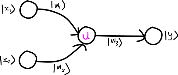
where we make the weights quantum states, and the weights are multiplied onto
the inputs as a dot-product. This would require that the weight state is the
same size as the input state; but that should be possible because we’re the
ones building the network structure.
Update: The idea about multiplying weights in didn’t make any sense; a much more sensible idea would be to prepare something like |wi⟩⟨wi| and enact this on the input |xk and then apply the fixed unitary.
We could then not worry about learning unitary matrices, and analogously to standard neural networks, just pick some unitary U that “works well” in practice, maybe by just defining quantum analogues of some common activation functions, perhaps say the ReLU or ELU.
Overall I think that the quantum gradient descent algorithm should be useful for training neural networks, and maybe some cool things will come from it. There are some natural direct extensions of this work; namely to extend the implementation to the more practical variations.
1612.02806 - Quantum autoencoders for efficient compression of quantum data
This paper came out only a few days after the Wan et al paper that we covered above, that also discussed autoencoders, so I thought it was worth a glance to see if this team did things differently.
This paper again takes the approach of not concerning itself with weights and instead focuses on learning a good unitary matrix U with a specific cost function.
They take a different approach in how they build their unitaries. Here they have a “programmable” quantum circuit, where they consider the parameters defining this circuit as the ones that can be trained. Given that these parameters are classical, and loss function they calculate is classical, no special optimisation techniques are needed.
Final thoughts
It appears that the building blocks are being put together to start doing some serious work on quantum machine learning/quantum deep networks. Google and Microsoft are already heavily investing in quantum computers, Google in particular has something it calls the “Quantum A.I. Lab”, and there are even independent quantum computer manufacturing groups.
It seems like there are lots of options on which way to direct efforts in the quantum ML world, and with these recent developments on quantum ML techniques, the time appears to be right to be getting into quantum deep learning!
Appendix
More interesting quantum machine learning papers:
- 1611.09347 - Quantum Machine Learning (most recent review)
- 1610.08251 - Quantum-enhanced machine learning
- 1605.05370 - Training A Quantum Optimizer
- 1603.08675 - Quantum Recommender Systems
- 1512.06069 - Demonstration of quantum advantage in machine learning
- 1512.02900 - Advances in quantum machine learning
- 1611.08104 - Quantum Enhanced Inference in Markov Logic Networks
- 1609.02542 - Quantum-assisted learning of graphical models with arbitrary pairwise connectivity
- 1609.06935 - Quantum Neural Machine Learning - Backpropagation and Dynamics
- 1606.02318 - Solving the Quantum Many-Body Problem with Artificial Neural Networks
- even more: SciRate - quantum machine learning!
Here efficient means that the problem is in the complexity class caled P. Problems that are efficient for quantum computers are in the complexity class BQP. One of the main outstanding questions in the field is “Are quantum computers more powerful than classical ones?” and this can be phrased as comparing the class P and BQP.↩︎
“Something like” x here is a very informal term for the more formal statement that the running time is O(x). See Big O Notation for more.↩︎